Web Application
pyadps includes an interactive web interface built with Streamlit for processing RDI ADCP data without writing any code.
Launching the Application
pyadps-gui
The application opens in your default web browser at http://localhost:8501.
Processing Workflow
The sidebar lists all pages in order. Processing must be carried out sequentially — each page builds on the state saved by the previous one. Always start at Page 1 and work downward through the sidebar.
 1. Read File            →  Upload file and inspect metadata
 2. View Raw Data        →  Visualize unprocessed data
 3. Download Raw File    →  Export raw data (optional)
 4. Time Diagnostics     →  Correct time axis before processing
 5. Sensor Health        →  Validate and correct environmental sensors
 6. Signal Quality       →  Apply QC thresholds
 7. Profile Operations   →  Trim, cut bins, and regrid
 8. Velocity Processing  →  Velocity checks and magnetic correction
 9. Write File           →  Export processed data and config
10. Add-Ons              →  Auto processing and file combiner
Processing Guidelines
For the decision logic behind the steps that involve a judgment call — time diagnostics, sensor health, signal quality, and profile operations — see the processing pipeline flowchart on the front page.
Navigate in order. Go through every page, and every tab within a page, in sequence. Each page reads the state saved by the one before it, so skipping ahead can mean working from stale or incomplete data.
Refresh after revisiting an earlier page. If you go back to an earlier
page and change a value (a threshold, a cutoff, anything already applied
further down the pipeline), refresh the browser tab afterward. This is not
a browser-caching problem — Streamlit’s session state itself updates
correctly. The real cause is a known Streamlit issue
(streamlit/streamlit#6257):
content rendered before a page’s st.tabs() call can reset which tab is
currently selected, which is exactly what happens when you revisit a page
you’ve already configured. A refresh reliably clears it.
Page Reference
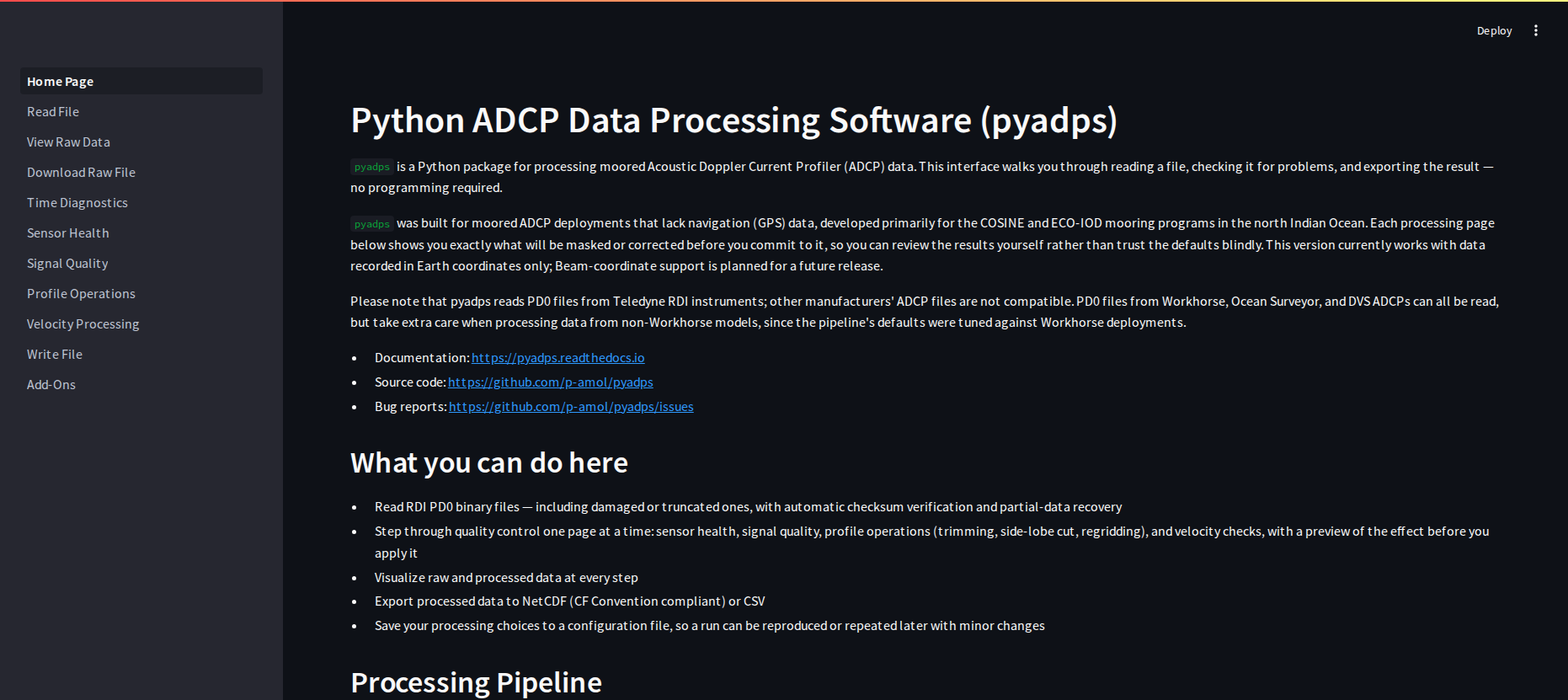
Home Page
Page 1: Read File
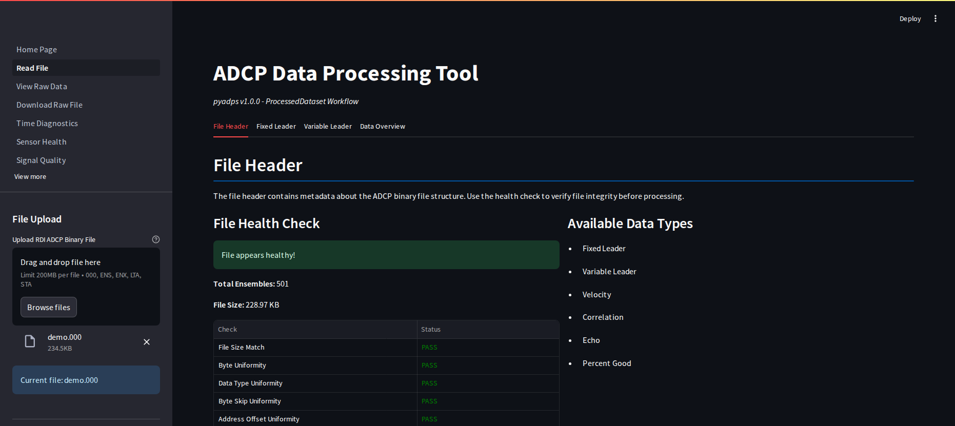
Upload an ADCP binary file and inspect its metadata. This page initialises
the ProcessedDataset that all subsequent pages use — always start here.
Tabs
Tab |
Description |
|---|---|
File Header |
Binary file structure and integrity check |
Fixed Leader |
System configuration, sensors, coordinate transform |
Variable Leader |
Time analysis, motion sensors, environmental sensors |
Data Overview |
Available data arrays and dimensions |
Tip
Use this page to catch problems early: whether the file is corrupted, whether BIT (built-in test) or Error Status Word results flag a sensor fault, whether the time axis is already irregular, and whether Fixed Leader fields (bin size, serial number, etc.) change unexpectedly partway through the deployment. Confirm the pre-deployment configuration matches what you expect before moving on.
Page 2: View Raw Data
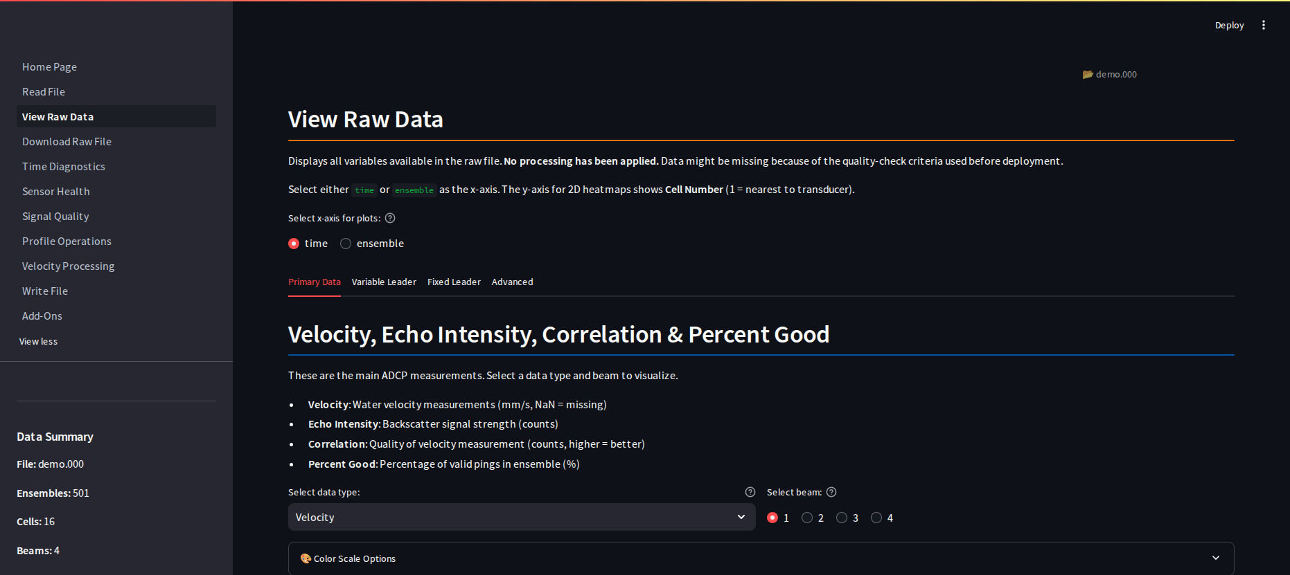
Visualise the raw dataset before any processing is applied.
Tabs
Tab |
Description |
|---|---|
Primary Data |
Velocity, echo intensity, correlation, percent good heatmaps |
Variable Leader |
Dynamic sensor measurements (heading, pitch, roll, temperature) |
Fixed Leader |
Static configuration values |
Advanced |
BIT results, ADC channels, Error Status Words |
Tip
Go through all the data at least once before processing. In the Primary Data tab, velocity should sit within the expected range; echo intensity, correlation, and percent good can reveal whether a beam is working. The Fixed Leader tab shows what changes over the deployment — a change in bin size or serial number partway through is a red flag worth investigating before you proceed.
Page 3: Download Raw File
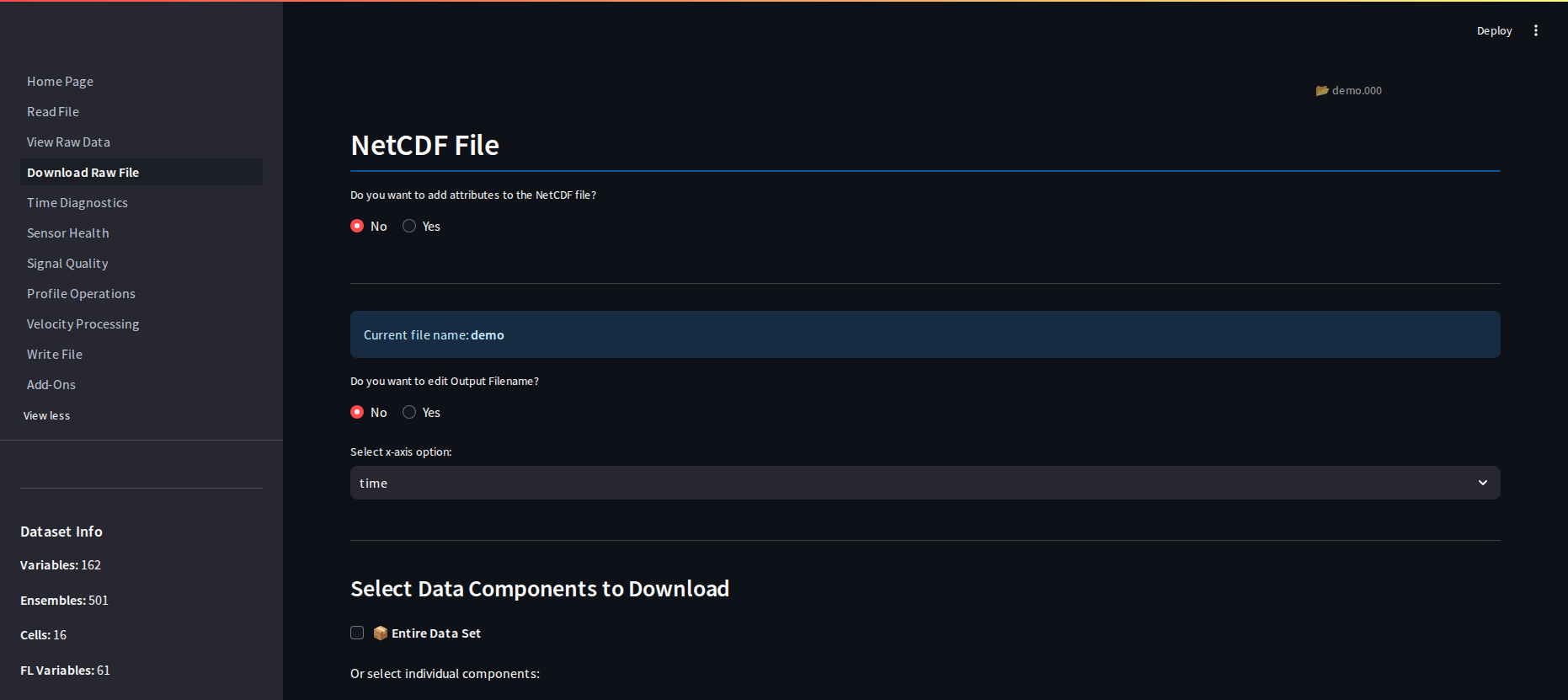
Export the raw dataset to NetCDF or CSV without any processing applied. This step is optional and can be skipped if you only need the processed output.
Tip
Choose ensemble or time as the index coordinate, and NetCDF or CSV as the output format. The data are saved as-is from the binary file, with no processing applied. Attributes entered here (e.g. latitude/longitude) can be reused on the final exported file, or picked up automatically to auto-fill the magnetic declination location on the Velocity Processing page.
Page 4: Time Diagnostics
Diagnose and correct the time axis before any QC processing begins.
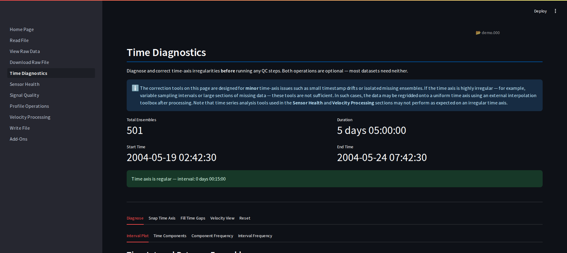
Tabs
Tab |
Description |
|---|---|
Diagnose |
Time interval statistics, gap detection, and component plots |
Snap Time Axis |
Round drifted timestamps to the intended recording interval |
Fill Time Gaps |
Insert synthetic ensembles to make the time axis uniform |
Reset |
Undo corrections and restore the original time axis |
Tip
Snap and Fill are built for minor issues — small timestamp drifts or a few isolated missing ensembles — and will refuse to apply a correction that exceeds the tolerance you set. For a heavily irregular time axis (variable sampling intervals, large gaps), don’t force it here: continue through the rest of the pipeline and fix the time axis with an external tool afterward. Either way, resolve what you can here first — Sensor Health and Velocity Processing’s time-series tools may not behave as expected on an irregular time axis.
Page 5: Sensor Health
Validate environmental sensors and optionally replace pressure, salinity, and temperature with external data (e.g. from a co-deployed CTD).
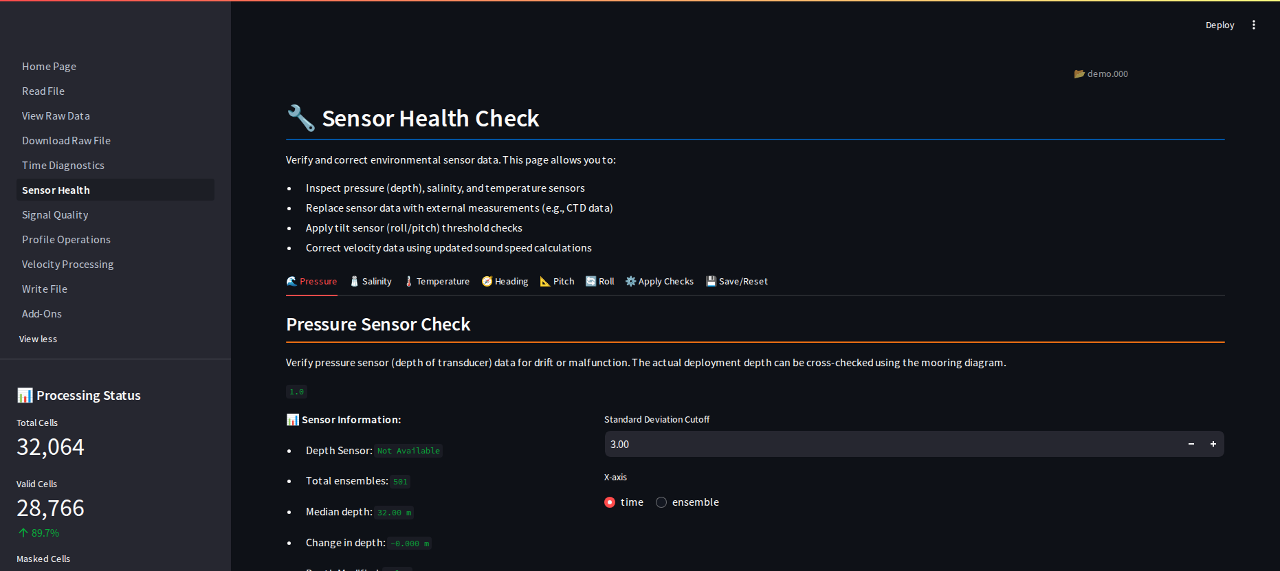
Tabs
Tab |
Description |
|---|---|
🌊 Pressure |
Transducer depth sensor with drift analysis |
🧂 Salinity |
Salinity sensor — replace with fixed value or CSV |
🌡️ Temperature |
Temperature sensor with drift analysis |
🧭 Heading |
Heading sensor visualisation |
📐 Pitch |
Pitch sensor with threshold indicator |
🔄 Roll |
Roll sensor with threshold indicator |
⚙️ Apply Checks |
Configure roll/pitch thresholds and sound speed correction |
💾 Save/Reset |
Commit or undo changes |
Tip
Verify each sensor makes sense for the deployment configuration. Roll and pitch have explicit thresholds that flag out-of-range tilt automatically; pressure, salinity, temperature, and heading have no automated pass/fail check, so inspect their plots directly. If a sensor looks bad, replace it with external data (e.g. a co-located CTD) where available; if no alternate source exists, fall back to a fixed value appropriate to the deployment.
Page 6: Signal Quality
Apply signal quality thresholds to mask low-quality data.
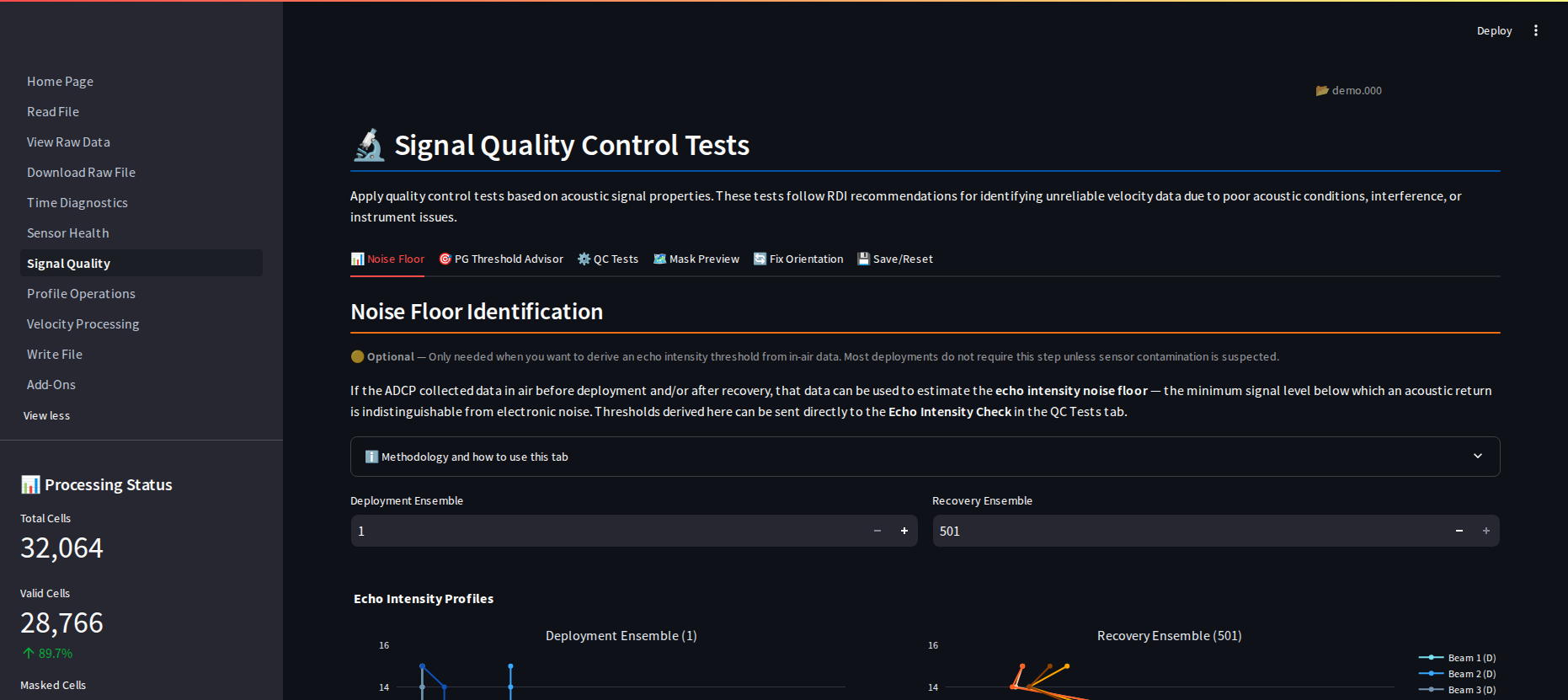
Tabs
Tab |
Description |
|---|---|
📊 Noise Floor |
Echo profiles for identifying the noise floor |
🎯 PG Threshold Advisor |
Recommend a percent-good cutoff for a target precision |
⚙️ QC Tests |
Configure correlation, echo, error velocity, percent good, false target |
🗺️ Mask Preview |
Before/after mask comparison |
🔄 Fix Orientation |
Correct beam direction (Up/Down) |
💾 Save/Reset |
Commit or undo changes |
Tip
Work through each check in turn:
Echo Intensity — decide whether to apply a threshold at all. If you have in-air data (recorded before deployment or after recovery), use the Noise Floor tab to identify the threshold automatically; otherwise enter one manually.
Percent Good — if you want to apply this threshold, use the PG Threshold Advisor tab to get a cutoff recommendation for your target precision, rather than guessing a value.
Correlation / Error Velocity / False Target — these default to values read from the instrument’s own pre-deployment commands, so check the pre-deployment values shown on the QC Tests tab before changing anything. That said, some factory defaults are known to be too lenient (the default error velocity threshold, for example) and are worth tightening.
Orientation — if the orientation sensor has gone bad, correct the beam direction on the Fix Orientation tab.
Of these, Percent Good deserves particular care — it’s the most direct indicator of solution reliability.
Page 7: Profile Operations
Modify the profile structure — trim deployment/recovery periods, remove side-lobe contaminated bins, and optionally regrid to a regular depth grid.
Note
Apply profile operations after signal quality checks. Regridding changes the dataset structure and invalidates cell-based masks from earlier steps.
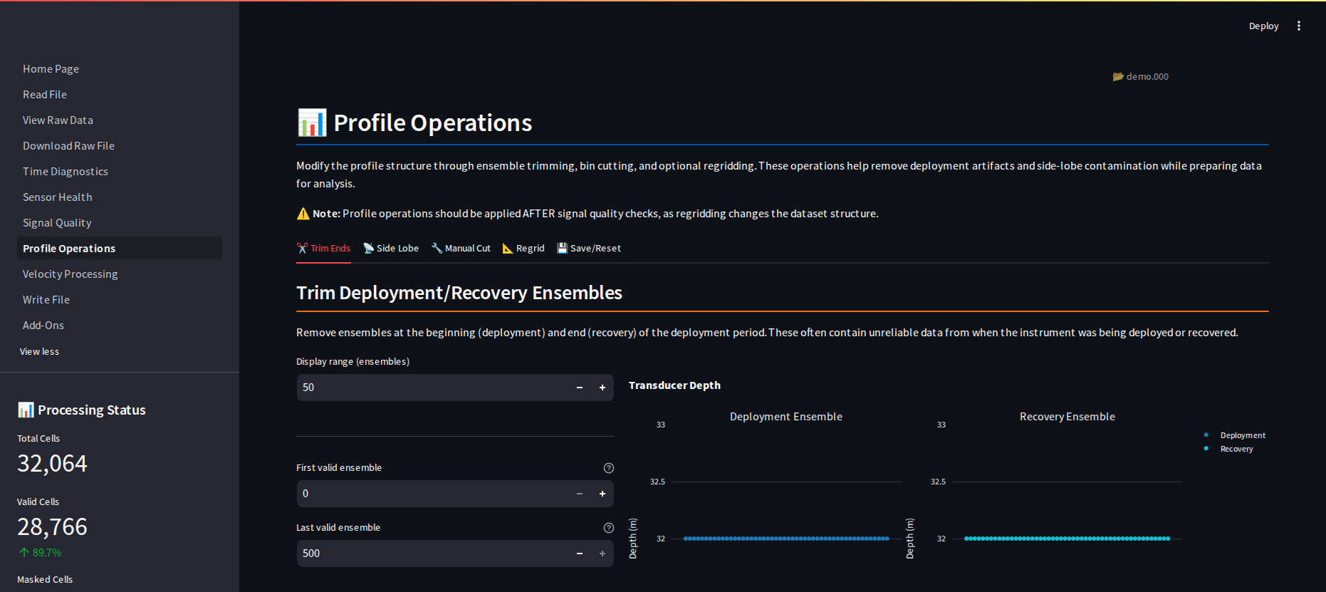
Tabs
Tab |
Description |
|---|---|
✂️ Trim Ends |
Remove ensembles from deployment/recovery periods |
📡 Side Lobe |
Physics-based side lobe contamination removal |
🔧 Manual Cut |
Cut arbitrary rectangular regions of cells and ensembles |
📐 Regrid |
Interpolate to a regular depth grid |
💾 Save/Reset |
Commit or undo changes |
Tip
Trim the pre-deployment and post-recovery periods (data collected in air) first. If the beam signal reaches the surface or the bottom, remove the affected bins with the Side Lobe cut, and use Manual Cut for any other suspect cells you’ve identified. Do Regrid last — once the data is regridded to the pressure sensor’s depth grid, cell-based masks from earlier steps no longer apply.
Page 8: Velocity Processing
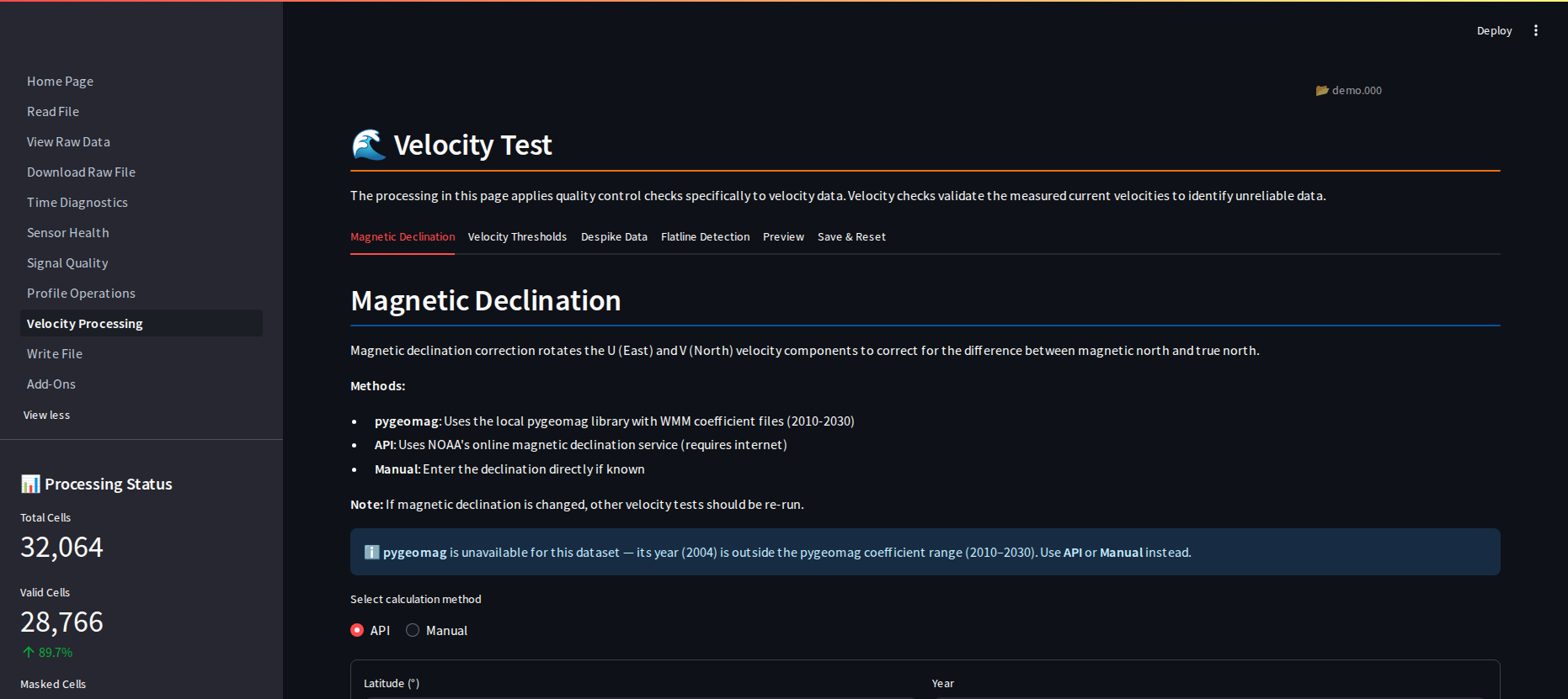
Apply velocity-specific quality control and magnetic declination correction.
Tabs
Tab |
Description |
|---|---|
Magnetic Declination |
Apply declination correction to U/V components |
Velocity Thresholds |
Set per-component cutoffs (U, V, W) |
Despike Data |
Median-filter spike detection |
Flatline Detection |
Detect frozen/stuck sensor values |
Preview |
View mask impact before committing |
Save & Reset |
Commit or undo changes |
Tip
This is the final check on the velocity data itself. All four steps are independently optional — apply whichever apply to your deployment, in any combination. Magnetic Declination uses the deployment’s latitude/longitude — auto-filled here if you entered it on the Download Raw File page. Velocity Thresholds, Despike, and Flatline Detection then catch out-of-range values, spikes, and frozen/stuck readings respectively.
Page 9: Write File
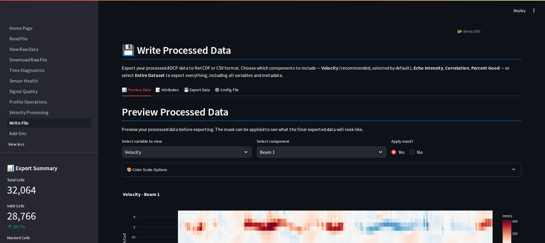
Export the processed dataset and save the processing configuration.
Tabs
Tab |
Description |
|---|---|
📊 Preview Data |
Visualise processed data with QC mask applied |
📝 Attributes |
Add custom metadata (cruise number, location, etc.) |
💾 Export Data |
Choose components and export as NetCDF or CSV |
⚙️ Config File |
Download |
The exported config.ini can be used with the Auto Processing tool (Page 10)
to reprocess data with adjusted parameters without repeating the full workflow.
Tip
Export Data lets you pick which components to include — Velocity (checked
by default), Echo Intensity, Correlation, Percent Good — or check Entire
Dataset to export everything instead (equivalent to a full raw dump,
overriding the individual checkboxes). Velocity variable names default to
the short form (u, v, w); switch to CF-style long names
(zonal_velocity, meridional_velocity, vertical_velocity) or enter
your own if you prefer — either way the file stays CF-compliant, since CF
Convention governs attribute values, not variable names. Exported NetCDF
filenames end in _PRO.nc.
Download the final processed data and the config.ini together — the
config file records every setting you used, so the run can be reproduced
or repeated later with minor adjustments instead of redoing the whole
workflow by hand.
Page 10: Add-Ons
Supplementary tools for batch reprocessing and combining multi-segment files.
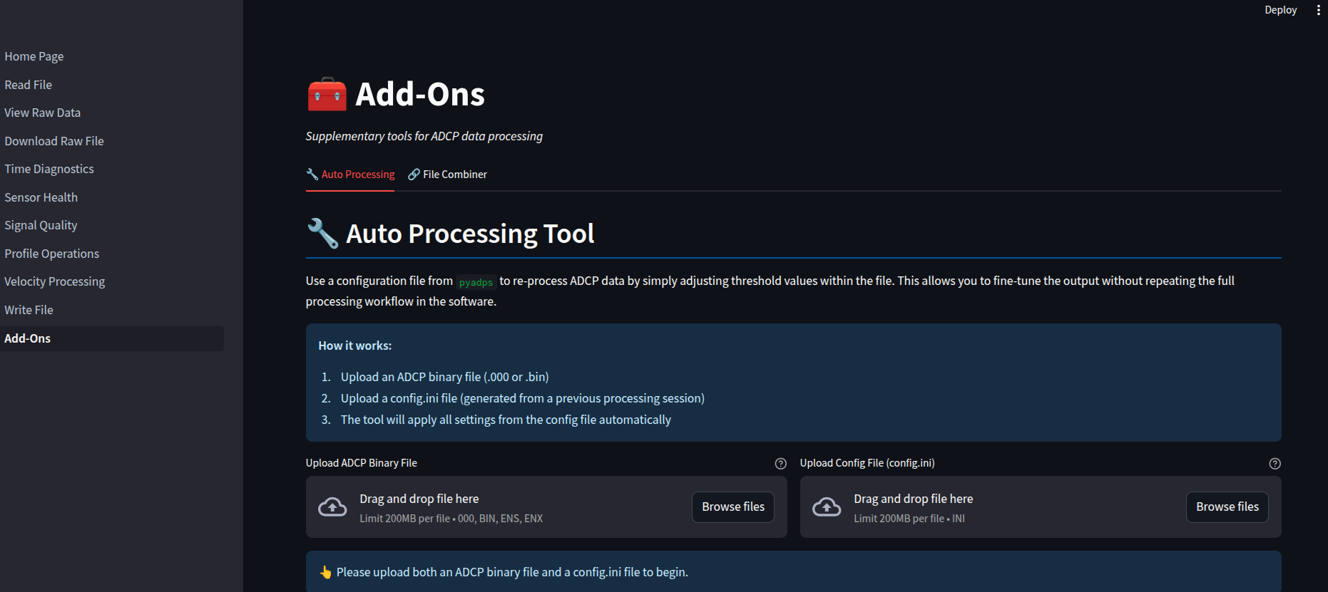
Auto Processing
Reprocess an ADCP file using a previously saved config.ini.
File Combiner
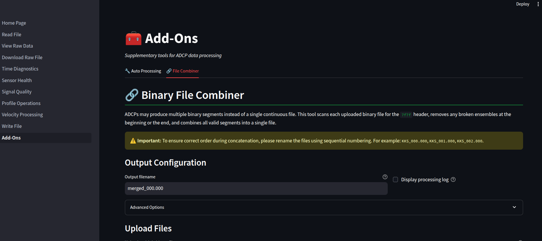
Merge multiple sequential ADCP binary files into a single file.
Note
When combining files, rename them with sequential numbering before uploading
(e.g. KKS_000.000, KKS_001.000, KKS_002.000) to ensure correct ordering.
See Also
Quick Start — Python API quick start
Processing Module — Processing module reference